EEG Signal Classification
An end‑to‑end workflow for EEG‑oriented biosignal classification, turning raw synchronized brain activity recordings into leakage‑safe training splits and reproducible model evaluation artifacts from the UC Berkeley BioSense dataset.
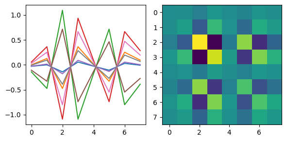
IMAGINATION: EEGImage
Imagination (EEGimage) converts EEG raw values, statistical features, power bands, and Fourier transforms into visual representations into 2D arrays (images). Then, trains a convolutional neural network to classify these images into mental states. The goal is to leverage spatial patterns in the data that may be more easily captured by CNNs:
Project Summary
This project addresses the complete lifecycle of EEG classification: data ingestion from synchronized multi-sensor exports, preprocessing and feature engineering, subject-aware splitting to reduce leakage risk, and model training with reproducible evaluation artifacts.
The core challenge lies not in raw model accuracy, but in maintaining transparency across failure modes including extreme class imbalance (31.6x largest vs. smallest), sparse per-class support, subject shift, and coarse temporal feature summaries. The pipeline logs per-subject performance, confidence intervals, and diagnostic reports to enable systematic diagnosis of model behavior. Project repository available on GitHub.
Project Highlights
Key contributions to this reproducible pipeline include:
- Leakage‑Safe Subject-Aware Splitting: Train on 21 subjects, test on 5 unseen subjects, eliminating data leakage while maintaining realistic subject-shift conditions.
- Imbalanced Multiclass Handling: Class weights computed from training distribution, systematically logged to diagnose why minority classes remain difficult to classify.
- Reproducible Feature Pipeline: Aggregate statistics, bandpower snapshots, and curated feature sets exported with train/val/test splits and summary metadata.
- Diagnostic Model Reports: Per-subject performance matrices, failure case analysis, and confidence intervals to expose subject-level generalization gaps.
- End-to-end Automation: Python scripts for preprocessing, splitting, training, and evaluation with saved artifacts (plots, metrics, configurations).
Technical Workflow
1) Data Ingestion
Raw sensor exports from UC Berkeley BioSense are synchronized across 26 subjects. Multi-modal biosignals include acceleration, blood volume pulse, electrodermal activity, heart rate, inter-beat interval, and temperature.
2) Preprocessing & Feature Engineering
Signals are cleaned, artifacts removed, and transformed into tabular features: statistical summaries (mean, std, quantiles) and bandpower snapshots across frequency bands. Unlabeled records are optionally dropped to ensure label integrity.
3) Subject-Aware Splitting
Group K-Fold cross-validation stratified by subject prevents train-test subject leakage. Splits yielded train (21 subjects), validation (overlapping), and test (5 held-out subjects) with balanced class representation within each fold.
4) Model Training & Evaluation
Models trained with class weights and evaluated using macro F1, AUC-OvR, and per-subject accuracy matrices. Reports capture per-label support, confidence intervals, and failure modes to diagnose generalization challenges.
Data Characteristics & Model Compensation
The figures below reveal why this dataset is challenging and how the pipeline adapts to extreme imbalance.
Class Weights Distribution
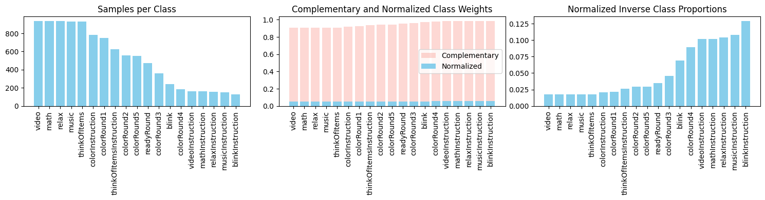
Why it matters: This plot shows how strongly minority classes must be upweighted in the loss function so the optimizer does not ignore them. Larger weights (taller bars) correspond to rarer classes. Without these adjustments, the model would converge on the majority class and achieve high accuracy with zero meaningful minority-class detection.
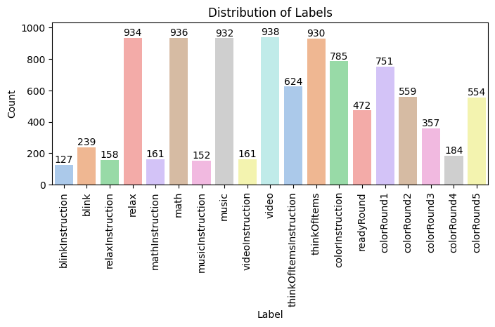
Label Distribution
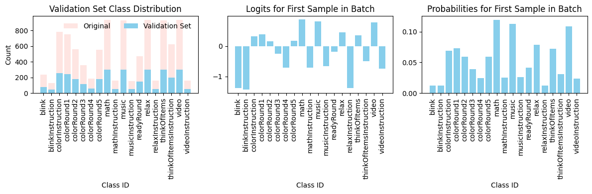
Why it matters: This distribution makes the long-tail imbalance problem explicit. The dataset has a 31.6× ratio between the most common and least common classes. Many fine-grained labels have <5 training examples, making it nearly impossible to learn robust decision boundaries for those classes without aggressive regularization and group-aware validation.
Impact on Model Behavior
These two visualizations together expose why macro-level metrics (macro F1, macro AUC) are difficult to optimize: the model must balance learning from the majority class (where signal is strong) while simultaneously pushing decision boundaries to support tiny minority classes (where signal may be weak and support is sparse). Class weighting helps, but cannot overcome the fundamental data scarcity problem.
The solution is not to expect perfect accuracy across all classes, but to:
- Track per-subject and per-class performance separately to understand where the model fails.
- Use subject-aware splitting to diagnose whether failures are due to subject shift or insufficient data.
- Log confidence intervals and minority-class recall to prioritize improvements where they matter most.
- Design the pipeline to be interpretable, not just accurate—so practitioners can reason about model behavior.
Challenges & Lessons Learned
Extreme Class Imbalance
The training set has a 31.6× imbalance ratio between largest and smallest classes. Even with aggressive class weighting, minority labels receive few positive examples. This limitation is addressed via class weights in the loss function and documented in diagnostic plots.
High-Dimensional Feature Space
Aggregate statistics and bandpower snapshots capture signal characteristics but may miss fine-grained temporal dynamics. Feature selection and dimensionality reduction techniques are logged to improve model interpretability.
Subject-Level Domain Shift
Training on 21 subjects and testing on 5 new ones introduces realistic but challenging subject shift. Per-subject performance matrices reveal where the model generalizes well and where it struggles, enabling targeted domain adaptation strategies.
Sparse Per-Class Support
Many fine-grained labels have very few training examples. This sparsity makes learning robust one-vs-rest boundaries difficult. The pipeline explicitly tracks per-label support to distinguish between true model failure and insufficient data.
Reproducible Artifacts
All outputs are versioned and reproducible, enabling audit trails and model comparison:
- Processed Datasets: features_with_split.csv, train/val/test splits, summary.json
- Model Reports: Metrics, per-subject accuracy matrices, training history
- Diagnostic Plots: Class weight distributions, label distributions, model outputs
- Configuration Logs: Feature definitions, split metadata, model hyperparameters